MATLAB Tutorial - Der Einstieg für Ingenieure
Die MATLAB Plattform des Unternehmens Mathworks wird in Industrie und Forschung für numerische Simulation sowie Datenanalyse eingesetzt. Das vorliegende Tutorial vermittelt Grundlagen der MATLAB-Sprache und Entwicklungsumgebung. Die Syntax (Variablen, Operatoren, Eingabe, Ausgabe, Arrays, Matrizen, Funktionen und Plots) wird mit Hilfe einfacher Beispiele veranschaulicht, die interaktiv, als MATLAB-Skript oder Live Script ausgeführt werden können.
Motivation
Mathematische Entwicklungsumgebungen wie MATLAB oder Octave bieten Unterstützung für die analytische und numerische Lösung von Problemen, die mit mathematischen Modellen gelöst werden können. MATLAB verbirgt Implementierungsdetails und die zugrundeliegende Komplexität der Probleme. Ingenieure können sich auf die Modellierung eines Problems wie z.B. Wärmeleitung oder Konvektions-Diffusionsgleichung konzentrieren und mittels vorhandener Solver Lösungen erzeugen und visualisieren. Ebenso ist mit MATLAB jedoch auch die Entwicklung eigener Solver und benutzerdefinierter Visualisierungen möglich.
Warum MATLAB?
MATLAB bietet umfangreiche Funktionen zur Lösung numerischer Probleme, die gängige technische Aufgabenstellungen modellieren. Als Beispiel: mit den MATLAB ODE (Ordinary Differential Equation)-Solvern für gewöhnliche Differentialgleichungen kann man eine Vielzahl zeitabhängiger dynamischer Probleme lösen, z.B. Schwingungsprobleme oder Bevölkerungsdynamik beschreiben. Die PDE (Partial Differential Equation)-Toolbox bietet Funktionen zum Lösen partieller Differentialgleichungen, wie zum Beispiel im Bereich der Wärmeleitung oder Wellengleichungen. Die Toolboxen und Funktionen sind gut dokumentiert und es sind viele Beispiele verfügbar, die man als Ausgangspunkt für eigene Skripte verwenden kann.
Warum Octave?
Octave ist eine Entwicklungsumgebung für mathematische und numerische Aufgaben, kostenlos verfügbar, und von der Funktionalität her mit MATLAB vergleichbar. Die Software ist weniger elegant als MATLAB, jedoch kostenlos verfügbar, mit derselben grundlegenden Funktionalität, und kann verwendet werden, um die Grundlagen der MATLAB-Syntax zu erlernen.
Übersicht
Das Tutorial ist in zehn Abschnitte gegliedert, die zunächst die Bedienung der MATLAB-Entwicklungsumgebung erläutern, danach die ersten Codezeilen, die Deklaration von Variablen, Eingabe und Ausgabe, Programmablaufsteuerung mit Verzweigungen und Schleifen, Arrays, Matrizen und Funktionen sowie das Erstellen zwei- und dreidimensionaler Grafiken.
2 Erste Zeilen in MATLAB
2-1 MATLAB-Befehle clear clc close all
2-2 Hello World-Programm interaktiv und als Skript
2-3 Kommentare
2-4 Variablen und Datentypen8 Funktionen
8-1 Globale Funktionen
8-2 Lokale Funktionen
8-3 Anonyme Funktionen9 Plotting in MATLAB
9-1 2D-Plots mit plot
9-2 3D-Plots mit surf
1 MATLAB Umgebung
Um MATLAB verwenden und MATLAB Skripte ausführen zu können, ist eine funktionierende MATLAB oder Octave Installation erforderlich. Eine MATLAB Testversion kann auf der Mathworks Webseite heruntergeladen werden. Falls Sie Student sind, stellt Ihre Hochschule Ihnen ggf. auf andere Art und Weise einen MATLAB-Zugang zur Verfügung.
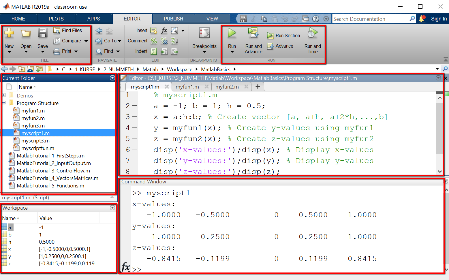
MATLAB's Editor-Tab ist in vier Fenster organisiert, die für die Entwicklung und Ausführung von Skripten verwendet werden. Die Anordnung dieser Fenster kann über das Layout-Menü angepasst werden.
- Datei-Browser: zeigt die Ordner und Dateien an, die MATLAB-Skripte enthalten. Hier werden neue Ordner und Skripte erstellt.
- Workspace: zeigt die Variablen und Funktionen der laufenden Skripte an.
- Editor: zeigt den Inhalt der Skript-Dateien an. Hier wird der MATLAB-Quellcode erstellt.
- Kommandofenster (Command Window): zeigt die MATLAB-Befehle an, wird für die Eingabe und Ausführung von Befehlen verwendet, sowie als allgemeines Ausgabefenster.
MATLAB kann auf verschiedene Arten verwendet werden:
- Interaktiver Modus: MATLAB wird im interaktiven Modus verwendet, indem man Befehle direkt in das Kommandofenster eingibt. Die Ausgabe wird ebenfalls im Kommandofenster angezeigt. Der interaktive Modus ist nützlich für kleinere Programme und um Codefragmente zu testen.
- MATLAB Skripte: Größere MATLAB-Programme sind Sammlungen von MATLAB-Skripten, die in einem gemeinsamen Ordner gespeichert werden. Dieser Ordner kann an einem beliebigen Speicherort abgelegt werden, muss jedoch zum MATLAB Pfad hinzugefügt werden, mit Hilfe des HOME > Set Path Menüpunktes.
- MATLAB Live Script: Live Scripts bieten erweiterte Funktionalität für Inline-Dokumentation. Sie haben die Dateiendung *.mlx und bestehen aus Codezellen, die den ausführbaren Code enthalten, und Markdownzellen, die formatierte Erläuterungen des Codes speichern. Die Erstellung und Verwendung von Live Scripts wird im nächsten Teil des Tutorials: MATLAB Live Scripts erstellen und verwenden gezeigt.
Ein MATLAB-Skript ist eine Textdatei mit der Dateiendung *.m, die die Befehle des MATLAB-Programms enthält.
Die Namen von MATLAB-Skripten dürfen nur aus Zeichen, Zahlen und Unterstrich (_) bestehen.
Gültige Skript-Namen sind z.B. myscript1.m, myscript2.m, myfun1.m, myfun2.m, nicht gültig: myscript-1.m oder myscript+1.m.
MATLAB-Skripte werden mit Hilfe der Befehle des EDITOR > FILE Menüs erstellt: New, Open, Save,
und mit Hilfe der Befehle des EDITOR > RUN-Menüs ausgeführt: Run, Run and Advance, Run Section.
Besonders hervorzuheben ist der Befehl Run Section: damit kann man einen einzelnen Abschnitt eines Skripts ausführen,
wobei Abschnitte durch zwei Prozentzeichen %% markiert werden.
2 Erste Zeilen in MATLAB
MATLAB Befehle bzw. Anweisungen sind: Deklarationen und Zuweisungen von Variablen, Operationen mit Variablen, Eingabe- und Ausgabe-Befehle, Befehle für die Programmablaufsteuerung (Verzweigungen und Schleifen) und Funktionsaufrufe, die definierte Teilaufgaben ausführen. MATLAB Anweisungen können mit einem Semikolon beendet werden oder nicht. Falls am Ende einer Anweisung kein Semikolon steht, wird der Inhalt der jeweiligen Variablen automatisch ausgegeben. Falls am Ende einer Anweisung ein Semikolon steht, wird die Anweisung keine Ausgabe erzeugen.
2-1 MATLAB-Befehle clear clc close all
MATLAB verfügt über eine Reihe von Steuerungsbefehlen wie clear, clc und close all, mit deren Hilfe man das Verhalten der Entwicklungsumgebung steuern kann, insbesondere den Workspace und das Kommandofenster überschaulich und konsistent halten. Bei dem Entwickeln und neuer MATLAB-Skripte kann es nützlich sein, das neue Skript mit einer Zusammenstellung von Befehlen wie
clear; clc; close all;
format compact;
einzuleiten, damit bei erneuten Ausführungen des Skripts z.B. die Ausgabe zurückgesetzt wird und auch zuvor geöffnete Grafik-Fenster geschlossen werden.
- clear – Löscht die Variablen des Workspace. Man kann entweder alle oder nur ausgewählte Variablen löschen. Nützlich, wenn man mehrere Skripte entwickelt, und dieselben Variablen-Namen wiederverwendet.
- clc – Löscht den Inhalt des Kommandofensters, Befehle und Ausgabe. Nützlich bei Demos und Vorführungen, wo man mit einem leeren Fenster beginnen möchte.
- close all – Schließt alle offenen Grafikfenster.
- format compact – Zeigt den Inhalt des Kommandofensters kompakt an, mit weniger Leerzeilen. Mit format long werden alle Kommazahlen mit doppelter Genauigkeit (d.h. mit mehr Nachkommastellen) angezeigt.
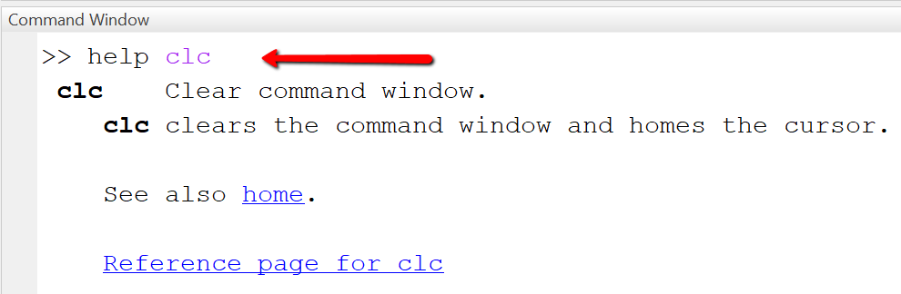
- help – Der Befehl help startet die MATLAB Hilfe. Falls man help gefolgt von dem Nahmen eines Befehls eingibt, wird die Hilfe zu dem betreffenden Befehl angezeigt.
Beispiel: Finde heraus, was der Befehl clc bewirkt.
Wenn wir "help clc" in das Kommandofenster eingeben, wird die Dokumentation des Befehls wie abgebildet angezeigt.
2-2 Hello-World-Programm interaktiv und als Skript
Ein Hello-World-Programm ist das kleinste lauffähige Programm in einer Programmiersprache und gibt den Text "Hello World" in die Default-Ausgabe (hier: das Kommandofenster) aus. Wir erstellen das Programm zunächst im interaktiven Modus und dann als Skript.
Interaktiver Modus
Im interaktiven Modus verwenden wir nur das Kommandofenster.
Befehle werden nach dem Prompt-Zeichen (>>) eingegeben und mit der ENTER-Taste bestätigt.
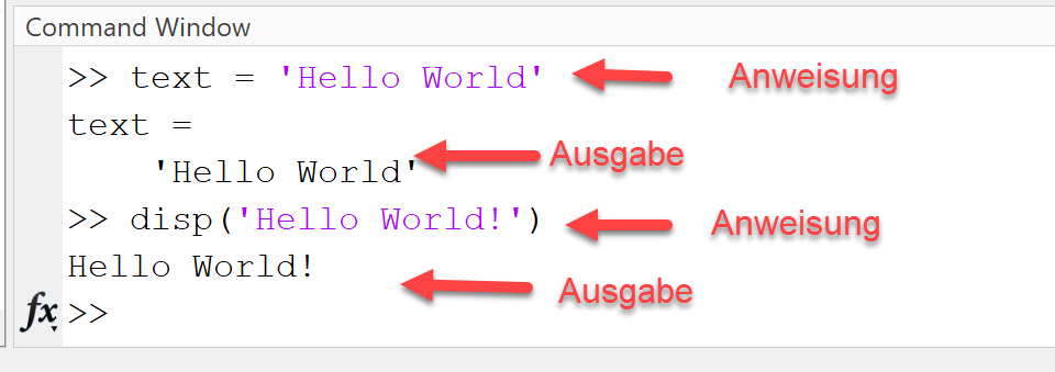
Wir geben den Befehl text='Hello World' in das Kommandofenster ein und bestätigen mit ENTER.
Wie in der Abbildung zu sehen ist, werden der Variablen-Name (hier: text) und ihr Inhalt (hier: Hello World)
im Kommandofenster angezeigt.
Als Nächstes geben wir den Befehl disp('Hello World') ein und bestätigen durch Drücken der ENTER-Taste.
Die Zeichenkette 'Hello World' wird wieder angezeigt, diesmal jedoch ohne den Namen der Variablen auszugeben.
Skript-Modus
Im Skript-Modus erstellen wir ein neues Skript mit den Namen test_hello.m,
schreiben die MATLAB-Befehle in das Skript, speichern die Datei und führen das Skript aus,
indem wir den RUN-Button in der Menüleiste anklicken.
Neue Skripte, Live Scripts, Funktionen und Klassen werden über den Menüpunkt New erstellt. Nach Erstellen der Skript-Datei, Editieren des Quellcodes und Ausführen des Skriptes sieht die MATLAB-Plattform wie unten abgebildet aus.
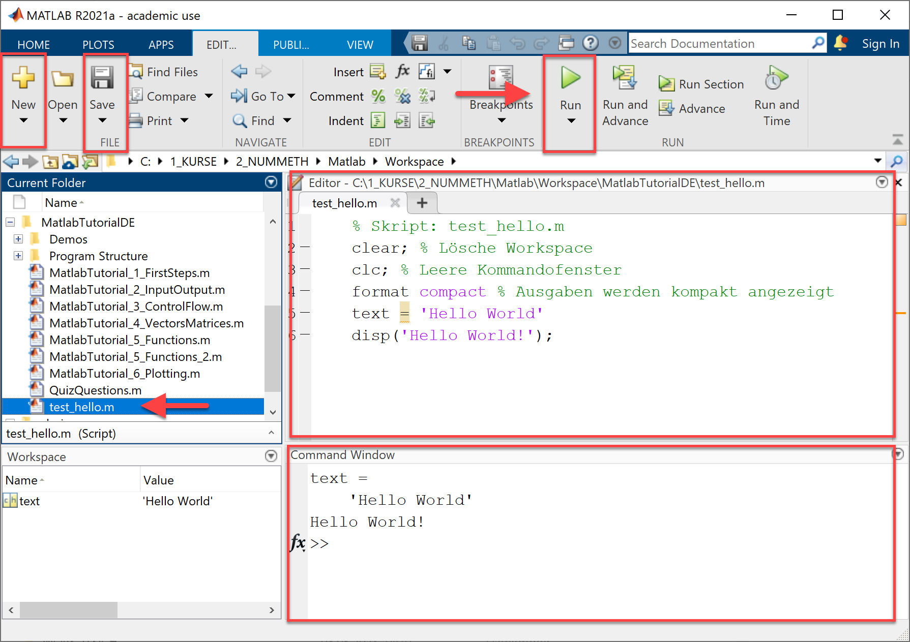
Der Code beginnt in Zeile 1 mit einem Kommentar (eingeleitet durch das "%"-Symbol), der den Namen der Skript-Datei angibt.
Die weiteren Zeilen sind zum besseren Verständnis ebenfalls kommentiert.
In Zeile 2 und 3 wird der Code für das Zurücksetzen des Workspace und des Kommandofensters eingefügt.
In Zeile 5 erstellen wir eine neue Variable "text" und weisen ihr den Wert 'Hello World!' zu.
In Zeile 5 geben wir den Text 'Hello World' mit Hilfe der Funktion disp() aus.
% Skript: test_hello.mclear; % Lösche Workspaceclc; % Leere Kommandofensterformat compact % Ausgaben werden kompakt angezeigttext = 'Hello World'disp('Hello World!');
2-3 Kommentare in MATLAB
Kommentare in MATLAB werden durch ein Prozentzeichen ("%"-Symbol) eingeleitet, gefolgt von Text. Kommentare werden für die Dokumentation des Quellcodes eingesetzt und vom System nicht ausgeführt. Zwei Prozent-Symbole "%%" markieren einen Abschnitt. Abschnitte können separat mit Hilfe des Menüpunktes RUN SECTION oder RUN AND ADVANCE ausgeführt werden, dabei ist ggf. die richtige Reihenfolge beim Ausführen von Abschnitten zu beachten.
%% Abschnitt 1% Kommentar 1: Erster Kommentar für Abschnitt 1text = 'Hallo zusammen!' % Weise der Variablen text einen Wert zu%% Abschnitt 2% Kommentar 2: Erster Kommentar für Abschnitt 2a = 10 % Weise der Variablen a den Wert 10 zub = 20 % Weise der Variablen b den Wert 20 zu
2-4 Variablen und Datentypen
Variable sind benannte Speicherplätze, in denen die Daten des Programms gespeichert werden. Variablen werden in MATLAB deklariert, sobald man ihnen einen Wert zuweist. Der Datentyp (Zahl, Zeichenkette etc.) wird automatisch durch MATLAB vergeben. Alle numerischen Werte in MATLAB (ganze Zahlen und Fließkommazahlen) werden intern als Fließkommazahlen mit doppelter Genauigkeit gespeichert. Die Kenntnis des Datentyps der Variablen ist wichtig, da der Datentyp die Menge der Operationen bestimmt, die man mit den Variablen ausführen kann. Zum Beispiel kann man eine ganze Zahl und eine Fließkommazahl addieren, nicht jedoch eine ganze Zahl und eine Zeichenkette.
Beispiel: Variablen verwenden
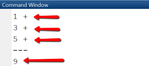
Das Beispiel zeigt, wie man Variablen deklariert und Operationen darauf ausführt.
Zu Beachten ist dabei, dass das +-Symbol unterschiedliche Operationen bezeichnet:
in Zeile 3 bezeichnet es die Addition von Zahlen, in Zeile 5, das Zusammenfügen von Zeichenketten.
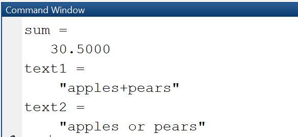
Nach Ausführen des Skriptes test_variables.m ist die Ausgabe im Kommandofenster wie abgebildet.
| Skript | Ausgabe |
|---|---|
|
|
Erläuterung des Quellcodes:
- Zeile 2: Deklariere zwei Variablen a, b und weise ihnen Werte zu. Da die Zuweisungen mit einem Semikolon abgeschlossen werden, erfolgt keine Ausgabe im Kommandofenster.
- Zeile 3: Addiere die beiden Variablen und speichere das Ergebnis in der Variablen sum.
- Zeile 4: Deklariere zwei String-Variablen s1 und s2.
- Zeile 5: Füge die beiden Zeichenketten in einer neuer Zeichenkette zusammen.
- Zeile 6: Ersetze das "+"-Zeichen mit der Zeichenkette ' or '.
Datentypen
MATLAB unterstützt die üblichen Datentypen, die intern durch Klassen abgebildet werden:
- Numerische Datentypen: int, single, double
- Boolesche Datentypen: logical
- Datentypen für Zeichen und Zeichenketten: char, string
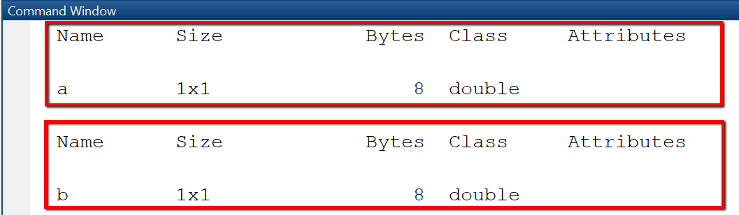
Um den Datentyp und die Größe von Variablen herauszufinden, werden die Befehle whos und class verwendet. Mit whos wird der Datentyp und die Größe von Workspace-Objekten zurückgegeben. Mit class wird der Datentyp bzw. die Klasse einer Variablen bestimmt.
| Skript | Ausgabe |
|---|---|
|
|
Zeichenketten bzw. String-Variablen
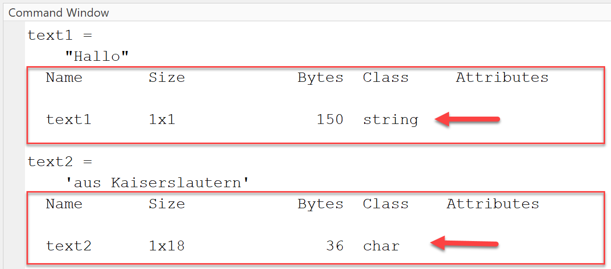
String-Variablen in MATLAB werden entweder durch die Klasse "string" oder als "character array" abgebildet. Wenn man eine Zeichenkette mit Hilfe von doppelten Hochkommas deklariert, z.B. text = "Hello", wird sie intern als ein Array aus einzelnen Zeichen hinterlegt. Wenn man eine Zeichenkette mit Hilfe von einfachen Hochkommas deklariert, z.B. text = 'Hello', wird sie intern als String abgelegt. Deklariert man Zeichenketten als String, stehen eine Reihe nützlicher Funktionen für die Textbearbeitung zur Verfügung.
| Skript | Ausgabe |
|---|---|
|
|
3 Eingabe und Ausgabe
Der Inhalt von Variablen kann im Workspace eingesehen werden oder im Kommandofenster ausgegeben werden.
Ausgabe im Kommandofenster
Es gibt drei Wege, um den Inhalt einer Variablen im Kommandofenster auszugeben.
- Semikolon weglassen: Schreibe den Namen der Variablen in eine neue Zeile, ohne abschließendes Semikolon. Oder: lasse das Semikolon am Ende einer Zuweisung weg.
- Verwende disp()-Funktion. Diese Funktion erwartet als Argument eine Variable, einen Vektor oder eine Matrix und gibt sie aus, ohne den Namen der Variablen mit auszugeben.
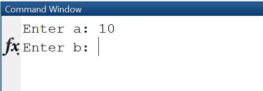
- Verwende fprintf()-Funktion. Diese Funktion erzeugt eine formatierte Ausgabe mit Hilfe von Platzhaltern für die einzufügenden Variablen. In unserem Beispiel wird an die Stelle wo %d steht, der Wert der Variablen a eingefügt.
Beispiel: Ausgabe im Kommandofenster
In diesem Beispiel wird die Summe zweier Variablen berechnet und das Ergebnis im Kommandofenster ausgegeben.
| Skript | Ausgabe |
|---|---|
|
Beim Ausführen des Skriptes test_output.m sieht die Ausgabe wie abgebildet aus. 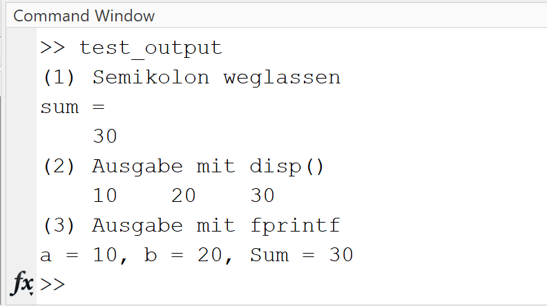
|
Eingabe über das Kommandofenster
Falls man ein Skript für nicht-technische Anwender schreibt, ist es nützlich, die Eingabeparameter über das Kommandofenster oder einen Eingabedialog abzufragen. In das Kommandofenster eingegebene Werte können mit Hilfe der input(prompt)-Funktion gespeichert werden.
| Skript | Ausgabe |
|---|---|
|
|
Eingabedialog erstellen
Ein Eingabedialog kann wie abgebildet mit Hilfe der Funktion inputdlg erstellt werden. Die Funktion erwartet vier Argumente:
- prompt – die Beschriftungen (Labels) der Eingabefelder
- dlgtitle – der Titel des Dialogfensters
- windowsize – die Größe des Dialogfensters
- definput – gibt den Default-Wert der Eingabefelder an. Das Argument für definput muss dieselbe Anzahl an Elementen haben wie prompt.
Die Funktion gibt ein Array aus Zeichenketten "answer" zurück, das die eingegebenen Werte speichert.
| Skript | Ausgabe |
|---|---|
|
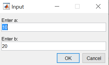
|
4 Programmablaufsteuerung
Die Befehle zur Programmablaufsteuerung werden verwendet, um abhängig von einer Bedingung den einen oder anderen Codeabschnitt auszuführen (bedingte Verzweigungen, if-else), oder um einen Codeabschnitt mehrfach zu wiederholen (while-loop, for-loop). Diese Befehle werden auch unter dem Begriff Kontrollstrukturen zusammengefasst, da sie den Programmablauf steuern bzw. kontrollieren. Kontrollstrukturen sind mehrzeilige Befehle, die mit dem Schlüsselwort end abgeschlossen werden müssen, um das Ende des Codeblocks anzuzeigen.
4-1 Verzweigungen
Eine bedingte Verzweigung ist eine Kontrollstruktur, die festlegt, welcher von zwei (oder mehr) Anweisungsblöcken, abhängig von einer (oder mehreren) Bedingungen, ausgeführt wird. Bedingte Verzweigungen werden in MATLAB, wie in fast allen Programmiersprachen, mit der if-else-Anweisung beschrieben. Das Schlüsselwort elseif bedeutet: "Wenn die vorherigen Bedingungen nicht zutreffen, versuche es mit dieser Bedingung" und das Schlüsselwort "else" fängt alles ab, was von den vorhergehenden Bedingungen nicht erfasst wird.
Beispiel: Ausgabe eines Textes abhängig von der Größe der eingegebenen Zahl
In diesem Beispiel wird der Anwender um die Eingabe eines Alters gebeten. Abhängig von der Größe der
eingegebenen Zahl erfolgt eine Ausgabe ins Kommandofenster.
In Zeile 6 wird die Bedingung "a < 2" ausgewertet: falls sie wahr ist, wird die Anweisung in Zeile 7 ausgeführt
und der Programmablauf wird in der ersten Zeile nach der if-else-Anweisung fortgesetzt, ansonsten wird
die Bedingung in Zeile 8 "a < 18" ausgewertet und bei Übereinstimmung die zugehörige Anweisung ausgeführt,
ansonsten wird die Anweisung im else-Teil ausgeführt.
| Skript | Ausgabe |
|---|---|
|
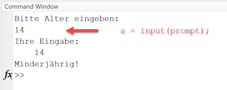
|
4-2 Schleifen
Schleifen ermöglichen es, Anweisungen wiederholt auszuführen, und zwar so lange, wie eine Ausführungsbedingung erfüllt ist. MATLAB verfügt über zwei Schleifenbefehle: while-Schleife und for-Schleife. Um den Kontrollfluss in Schleifen zu steuern, werden zusätzlich zu der Ausführungsbedingung die Anweisungen break und continue eingesetzt. Man kann in vielen Fällen eine for-Schleife als while-Schleife formulieren und umgekehrt. Sobald man verschachtelte Schleifen verwenden muss, z.B. um die Zeilen und Spalten einer Matrix auszulesen, ist die Verwendung von for-Schleifen knapper und übersichtlicher.
while-Schleife
Eine while-Schleife wiederholt die Anweisungen in einem Block, solange wie eine Ausführungsbedingung als wahr ausgewertet wird.
Beispiel: Berechne die Summe der ersten n Zahlen
In diesem Beispiel wird die Summe der ersten n Zahlen : sum = 1+2+...+n berechnet.
Zunächst wird in Zeile 2 eine Zählvariable i mit 1 initialisiert.
In Zeile 3 wird die Schleifenbedingung "i <= 5" überprüft.
Falls "wahr", werden die Anweisungen in Zeilen 4-6 ausgeführt:
gebe Wert von i aus, addiere Wert von i zur Summe hinzu, erhöhe Wert von i um 1.
Danach wird die Schleifenbedingung erneut überprüft und falls wahr, wird die Schleife wiederholt.
| Skript | Ausgabe |
|---|---|
|
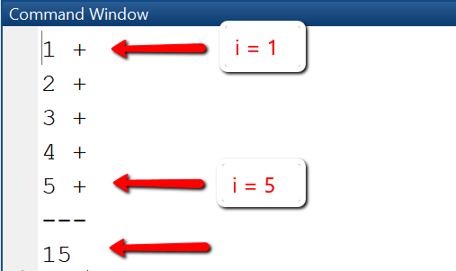
|
for-Schleife
Die for-Schleife erlaubt, Anweisungen wiederholt auszuführen, indem sie für festgelegte Zählvariablen Startwert, Endwert und Schrittweite festlegt.
Beispiel: Berechne Summe der ersten n Zahlen
Hier berechnen wir die Summe der ersten n Zahlen: sum = 1+2+...+n mit Hilfe einer for-Schleife. In Zeile 3 wird die Zählvariable i mit 1 initialisiert, während des Durchlaufs mit Schrittweite 2 erhöht und läuft bis zum Endwert n.
| Skript | Ausgabe |
|---|---|
|
|
5 Vektoren
Vektoren bzw. eindimensionale Arrays sind Listen von Datenobjekten, die im Arbeitsspeicher zusammenhängend abgelegt werden. Ein einzelnes Datenobjekt wird Element des Arrays genannt. In MATLAB können Vektoren als Zeilen- oder Spalten-Arrays deklariert werden, dies wird durch das Trennzeichen festgelegt, mit dem die Elemente aufgelistet werden. Zum Beispiel deklariert x = [1, 4, 9] einen Zeilen-Vektor, und x = [1; 4; 9] einen Spaltenvektor. Die Elemente eines Vektors werden über einen Index ausgewählt, d.h. ihre Position in der Liste, und in MATLAB beginnt dieser bei 1. Um das i-te Element aus einem Vektor x zu holen, schreibt man x(i) - hier mit runden Klammern.
5-1 Vektoren erstellen
Vektoren können auf unterschiedliche Arten erzeugt werden:
durch Aufzählen ihrer Elemente in eckigen Klammern, mit Hilfe von Funktionen (Doppelpunkt-Operator, linspace, repmat),
durch Zuweisen der Elemente in einer Schleife.
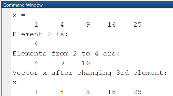
Beispiel: Erzeuge Vektor mit 5 Elementen
Wir erstellen einen Zeilenvektor mit 5 Elementen, geben das zweite Element des Vektors aus,
dann die Elemente zwei bis 4, und ändern den Wert des dritten Elementes.
| Skript | Ausgabe |
|---|---|
|
|
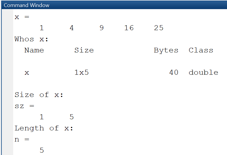
Beispiel: Bestimme Speichergröße und Länge eines Vektors
Mit Hilfe des Befehls whos, gefolgt vom Namen eines Vektors, können wir seine Dimensionen, seine Speichergröße und seinen Datentyp herausfinden,
hier: x ist eine Matrix mit einer Zeile und 5 Spalten (also ein Vektor), hat die Klasse double und verwendet 40 Bytes Speicherplatz.
| Skript | Ausgabe |
|---|---|
|
|
Vektoren aus Sequenzen
Bei der Entwicklung numerischer oder statistischer Anwendungen benötigt man oft regelmäßige Folgen (Sequenzen bzw. äquidistante Vektoren), wie z.B. 2, 4, 6, 8, 10 oder 0, 0.1, 0.2,..., 1. In MATLAB werden Sequenzen mit Hilfe des Doppelpunkt-Operators oder mit Hilfe der Funktion linspace erstellt. Der Ausdruck x = 1:n erzeugt den Vektor [1, 2, ..., n]. Allgemeiner erzeugt der Ausdruck x = a:h:b den Vektor [a, a+h, a+2*h, ..., b] mit Anfangswert a, Schrittweite h und Endwert b, und die Funktion x = linspace(a, b, n+1) denselben Vektor [a, a+h, a+2*h, ..., b], mit Schrittweite h = 1/n.
a = 0; b = 1; n = 10; h = 1/n;
x = linspace(a, b, n+1) % Ausgabe: 0, 0.1, 0.2,..., 1
x = a:h:b % Ausgabe: 0, 0.1, 0.2,..., 1
Vektoren aus Zufallszahlen
Ein weiterer Anwendungsfall zum Erstellen von Vektoren ist die Erzeugung von Zufallszahlen mit Hilfe der Funktionen rand, randi, randn. rand erzeugt gleichmäßig verteilte Zufallszahlen des Datentyps double in dem offenen Intervall (0, 1). Abhängig von den Argumenten, die beim Funktionsaufruf übergeben werden, wird eine Matrix, ein Spaltenvektor, ein Zeilenvektor, oder eine einzelne Zahl erzeugt. randi erstellt gleichmäßig verteilte ganzzahlige Zufallszahlen c, als Matrix, Spaltenvektor oder Zeilenvektor.
% 3x5 Matrix aus Zufallszahlen in (0, 1)r_mat = rand(3, 5)% Spaltenvektor aus 5 Zufallszahlen in (0, 1)r_col = rand(5, 1)% Zeilenvektor aus 5 Zufallszahlen in (0, 1)r_row = rand(1, 5)a = 10; b = 20; n = 5;% Zeilenvektor aus double-Zufallszahlen in (a, b)r_row_10_20 = rand(1, n)*(b-a) + a% Zeilenvektor aus int-Zufallszahlen in (a, b)r_int_10_20 = randi([a, b],1, n)
5-2 Vektoren verwenden
MATLAB unterstützt zwei Arten von Operationen für Vektoren: (1) Vektor-Operationen, d.h. mathematische Operationen entsprechend den Regeln der linearen Algebra
und (2) Array-Operationen, die elementweise durchgeführt werden.
Elementweise Operationen werden durch die Verwendung des Punkt-Operators (engl. dot-Operator) ausgezeichnet.
x * y bezeichnet die mathematische Multiplikation von Vektoren bzw. Matrizen, und funktioniert für Vektoren nur,
falls x eine 1xn Matrix bzw. ein Zeilenvektor und y eine nx1 Matrix bzw. ein Spaltenvektor ist.
x .* y bezeichnet die elementweise Multiplikation und funktioniert nur, wenn x und y Vektoren derselben Länge sind.
Vektor-Operationen und elementweise Operationen sind für Addition und Subtraktion gleich, so dass die Operatoren .* und .- nicht benötigt werden.
| Skript | Ausgabe |
|---|---|
|
|
6 Matrizen
Die Daten in vielen numerischen MATLAB-Programmen werden in ein- und zweidimensionalen Arrays gespeichert, d.h. Vektoren und Matrizen.
Variablen and Vektoren werden intern ebenfalls als Matrizen abgebildet.
6-1 Matrizen erstellen
Matrizen können auf unterschiedliche Arten erzeugt werden: (1) durch explizites Aufzählen ihrer Elemente in eckigen Klammern, (2) mit Hilfe vordefinierter MATLAB-Funktionen, oder (3) mit Hilfe von Schleifen.
(1) Erstelle Matrix durch Angabe der Elemente
Wird eine Matrix durch Angabe der Elemente erstellt, müssen Zeilen-Elemente mit einem Komma und Spalten mit einem
Semikolon getrennt werden.
(2) Erstelle Matrix mit Hilfe vordefinierter Funktionen
Viele mathematische Probleme verwenden Matrizen, die mit festgelegten Werten initialisiert werden, wie z.B.
die Einheitsmatrix, die 1en auf der Diagonale hat und sonst nur 0-Werte.
In MATLAB können Funktionen wie zeros(), ones() or eye() verwendet werden, um diese Matrizen zu definieren.
(3) Erstelle Matrix mit for-Schleifen
Das Erstellen einer Matrix mit for-Schleifen ist dann notwendig, wenn es sich um große Matrizen handelt,
und wenn die Größe und die Werte sich dynamisch ändern bzw. von Parametern abhängen.
In diesem Fall wird empfohlen, den maximal benötigten Speicherplatz mit Hilfe der zeros()-Funktion zu reservieren.
Auf die Elemente einer Matrix wird über einen Zeilenindex und einen Spaltenindex zugegriffen, beide beginnen bei 1. Mit dem Ausdruck A(i, j) wird auf das Element in Zeile i und Spalte j einer Matrix A zugegriffen. A(1, 1) ist das Element in Zeile 1 und Spalte 1, A(1, 2) das Element in Zeile 1 und Spalte 2 etc.
Beispiel: Erzeuge Matrix durch explizites Aufzählen
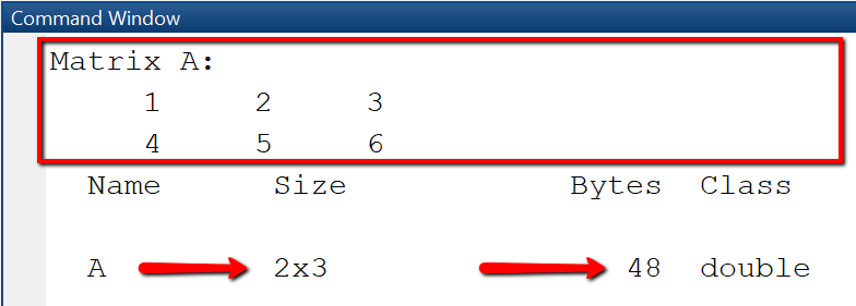
In diesem Beispiel erzeugen wir eine Matrix mit zwei Zeilen und drei Spalten, geben sie mit disp aus,
und bestimmen nachher Typ und Größe der Matrix mit whos.
Der whos-Befehl zeugt, dass eine 2x3 Matrix angelegt wurde und diese 48 Bytes Speicherplatz benötigt.
| Skript | Ausgabe |
|---|---|
|
|
Beispiel: Erzeuge Matrizen mit Hilfe von MATLAB-Funktionen
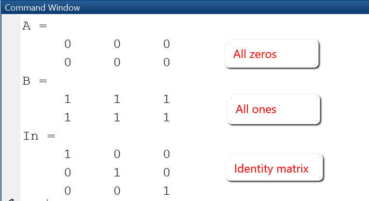
In diesem Beispiel erstellen wir drei Matrizen:
A1 ist eine Matrix mit m Zeilen und n Spalten, deren Elemente mit 0 initialisiert werden.
A2 ist eine Matrix deren Elemente alle mit 1 initialisiert werden.
I_n ist die Einheitsmatrix mit n Zeilen und n Spalten, mit 1 auf der Diagonale und 0 an allen anderen Positionen.
| Skript | Ausgabe |
|---|---|
|
|
Beispiel: Extrahiere Elemente aus einer Matrix
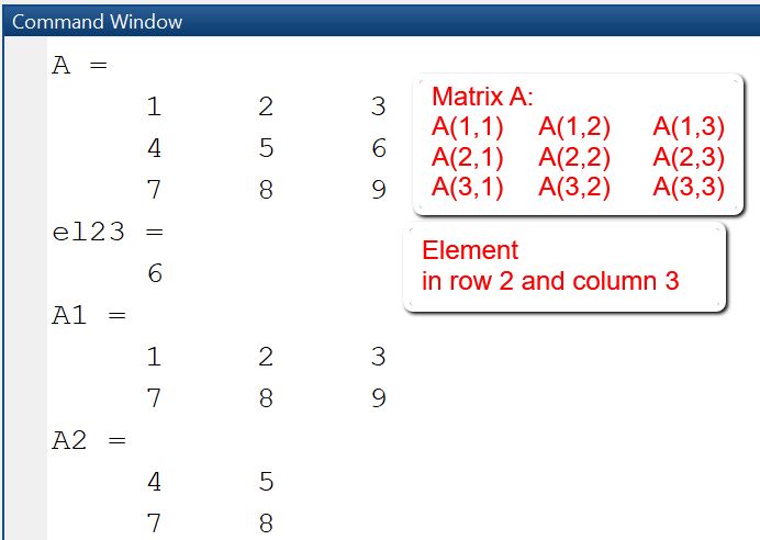
Die Elemente einer Matrix werden über ihren Index extrahiert.
In diesem Beispiel extrahieren wir das element mit Zeilenindex 2 und Spaltenindex 3 und speichern es in einer Variablen el23,
danach extrahieren wir die Zeilen 1 bis 3 und alle Spalten und speichern sie in einer neuen Matrix A1,
zuletzt extrahieren wird die Zeilen 2 und 3 und Spalten von 1 bis 2 uns speichern das Ergebnis is einer neuen Matrix A2.
| Skript | Ausgabe |
|---|---|
|
|
6-2 Matrizen verwenden
MATLAB unterstützt zwei Arten von Operationen für Matrizen: (1) Matrix-Operationen, d.h. mathematische Operationen entsprechend den Regeln der linearen Algebra
und (2) Array-Operationen, die elementweise durchgeführt werden.
Elementweise Operationen werden durch die Verwendung des Punkt-Operators (engl. dot-Operator) ausgezeichnet.
A * B bezeichnet die mathematische Multiplikation von Matrizen, und funktioniert nur, falls
die Anzahl der Spalten von A mit der Anzhl der Zeilen von B gleich sind, z.B. A eine mxn und B eine nxp Matrix ist.
A .* B bezeichnet die elementweise Multiplikation und funktioniert nur wenn A und B Matrizen mit derselben Anzahl von Zeilen und Spalten sind.
Matrix-Operationen und elementweise Operationen sind für Addition und Subtraktion gleich, so dass die Operatoren .* und .- nicht benötigt werden.
Beispiel: Operationen mit Matrizen
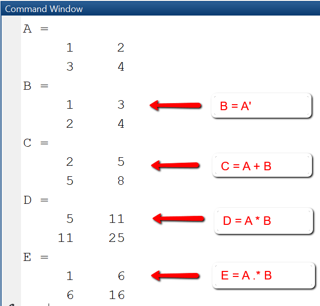
Dies Beispiel zeigt häufig verwendete Operationen mit Matrizen:
Transposition, Addition, Matrix-Multiplikation und elementweise Multiplikation.
Die Transponierte einer Matrix wird erstellt indem man A' schreibt, d.h. den Namen der Matrix, gefolgt von einem einfachen Hochkomma.
Alternativ kann auch die Funktion transpose() verwendet werden, und transpose(A) erzeugt die transponierte Matrix.
| Skript | Ausgabe |
|---|---|
|
|
7 Tabellen
MATLAB hat eine Datenstruktur namens table, die zum Speichern und Bearbeiten tabellenähnlicher Daten mit benannten Spalten ("Variablen") und ggf. auch Zeilennamen verwendet wird. Verschiedene Spalten können unterschiedliche Datentypen haben, aber die Elemente einer Spalte müssen denselben Datentyp haben. Auf Elemente kann sowohl über ihren Index als auch über Zeilen- und Spaltennamen zugegriffen werden. Die Datenstruktur table wird hauptsächlich für statistische Aufgaben verwendet, beispielsweise wenn Sie statistische Eigenschaften (Mittelwert, Standardabweichung, Min., Max.) der Variablen auswerten müssen. Tabellen sind auch nützlich, um schöne tabellarische Darstellungen von Daten zu erstellen, die aus Messungen oder dem Testen einer numerischen Methode stammen.
Tabellen können auf verschiedene Arten erstellt werden: zum einen aus Spaltenvektoren mit der table()-Funktion, zum anderen aus Arrays mit Hilfe der Funktion array2table() oder schließlich auch durch den Import von Daten aus einer Excel- oder CSV-Datei mittels readtable(). Die Eigenschaften einer Tabelle T wie DimensionNames, VariableNames, RowNames können mithilfe der T.Properties-Syntax ermittelt und festgelegt werden, wie in den folgenden Beispielen gezeigt.
7-1 Tabellen erstellen
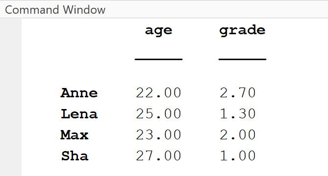
Eine Möglichkeit, eine Tabelle zu erstellen, besteht darin, bereits vorhandene Vektoren zu verwenden, diese müssen Spaltenvektoren sein und die gleiche Anzahl an Elementen haben. Die so erstellte Tabelle erhält automatisch die Namen der Vektoren als Spaltennamen.
| Skript | Ausgabe |
|---|---|
|
|
7-2 Tabellen ändern
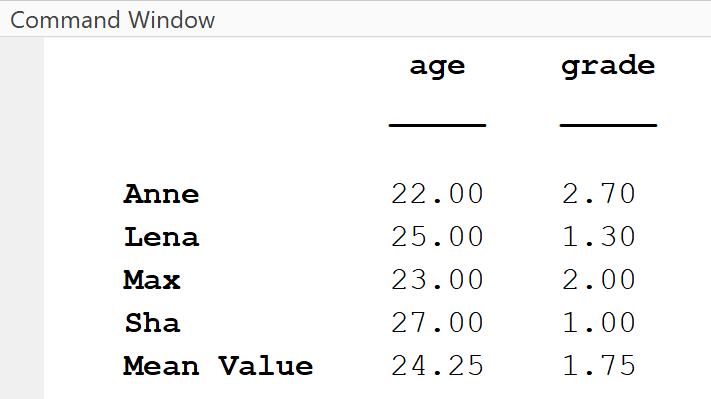
Tabellen können auf verschiedene Arten geändert werden: man kann Zeilen oder Spalten hinzufügen/entfernen/ersetzen, Daten extrahieren, statistische Werte für die Variablen (Spalten) der Tabelle berechnen oder die Variablen der Tabelle grafisch darstellen.
| Skript | Ausgabe |
|---|---|
|
|
8 Funktionen
Eine Funktion ist ein wiederverwendbarer Codeblock, der nur ausgeführt wird, wenn er aufgerufen wird. Funktionen werden einmal definiert und können dann beliebig oft aufgerufen werden. Man kann Daten oder sogenannte Parameter an eine Funktion übergeben. Eine Funktion kann auch Daten/Parameter zurückgeben. Funktionen kommen auf zweierlei Arten zum Einsatz: zum einen verwendet man vorhandene Funktionen, die von MATLAB bereitgestellt werden, um gewisse Aufgaben durchzuführen. Zum anderen entwickelt man eigene Funktionen für Teilaufgaben und strukturiert damit größere Programme.
MATLAB bietet vordefinierte Funktionen für Matrix-Bearbeitung (zeros, ones, eye, diag, ...), Erstellen von Grafiken( plot, surf, quiver, contour, ...) und zur Berechnung der Lösungen gewöhnlicher oder partieller Differentialgleichungen, sogenannte Solver (ode45, ode15s, pdepe, ...) und viele mehr. Um diese effizient nutzen zu können, ist ein Verständnis für die Funktionsweise und Verwendung von Funktionen erforderlich.
Benutzerdefinierte Funktionen können als globale, lokale oder anonyme Funktionen definiert werden, und die Art der Definition legt den Geltungsbereich fest:
- Globale Funktion: Funktion wird in einer eigenen m-Skript-Datei gespeichert.
- Lokale Funktionen: Funktion wird inline in dem Skript gespeichert, wo sie auch verwendet wird.
- Anonyme Funktion: Funktion wird als Variable des Typs type function_handle definiert.
8-1 Globale Funktionen
In den meisten Fällen ist es sinnvoll, die Funktion in ihrer eigenen Skript-Datei zu speichern.
Dies sichert die Wiederverwendbarkeit der Funktion in anderen Skripten.
Ein Funktions-Skript ist eine MATLAB m-Datei die nur die Definition einer Funktion enthält und nicht ausführbar ist.
Das Funktions-Skript muss denselben Namen haben wie die Funktion, die es enthält, z.B. muss eine Funktion mit dem Namen myfun1
in einem Skript mit dem Namen myfun1.m gespeichert werden.
Wird eine Funktion in einer eigenen Skript-Datei gespeichert, kann sie in anderen Skripten verwendet werden.
Der Name der Funktion sollte in diesem Fall eindeutig sein, um Fehler durch die Verwendung einer falschen
Variante der Funktion zu vermeiden.
Funktion definieren
Funktionen werden durch das Schlüsselwort "function", eingeleitet, gefolgt durch
outputargs = function_name(inputargs)
und enden mit dem Schlüsselwort "end".
Die Anweisungen, die zur Implementierung der Funktion gehören und die Beziehung zwischen den Eingabe-Parametern
inputargs und Ausgabeparametern outputargs herstellen, werden in den zwischen die erste "function"-Zeile und letzte "end"-Zeile
geschrieben.
Um die allgemeine Syntax einer Funktionsdefinition zu zeigen und eine Vorlage für eine neue Funktion zu erstellen
wird das New > Function-Menü im EDITOR-Tab verwendet.
Damit wir ein neues Funktion-Skript "untitled.m" für die Funktion "untitled" erstellt, mit zwei generischen Eingabe-Parametern
und zwei generischen Ausgabeparametern.
Ausgehend von dieser Vorlage können eigene Funktionen erstellt werden, indem der Name der Funktion, die Eingabe- und Ausgabeparameter,
sowie die Funktionsanweisungen angepasst werden.
function [outputArg1,outputArg2] = untitled(inputArg1,inputArg2)%UNTITLED Summary of this function goes here% Detailed explanation goes hereoutputArg1 = inputArg1;outputArg2 = inputArg2;end
Beispiel: Definiere und verwende eine Funktion myfun1
Im folgenden Beispiel erstellen wir eine Funktion myfun1, die als Eingabeparameter ein Array x erhält
und dafür die Funktionswerte y = x*exp(-x2) berechnet.
Der Quellcode zeigt die Funktionsdefiniton im eigenen Funktion-Skript.
Im Test-Skript myscript1.m erstellen wir zunächst einen Vektor aus äquidistanten Punkten x, berechnen durch einen
Funktionsaufruf der Funktion myfun1 die y-Werte und stellen die so erhaltenen (x,y)-Koordinaten mit Hilfe der plot-Funktion
grafisch dar.
MATLAB's plot-Funktion wird verwendet um 2D Liniengrafiken von Daten zu erstellen, die durch ihre x und y-Koordinaten gegeben sind. Die Funktion erwartet als Eingabe zwei Vektoren derselben Länge, die die x- und y-Koordinaten darstellen. Weiterhin können Formatierungsangaben als optionale Parameter mitgegeben werden, z.B. für die formatierung der Linienfarbe und -stärke, Titel und Legende sowie Beschriftung der Achsen.
| Skript | Ausgabe |
|---|---|
|
Funktion-Skript myfun1.m
Test-Skript myscript1.m
|

|
8-2 Lokale Funktionen
Funktionen, die nur in einem einzigen Skript verwendet werden, können als lokale Funktionen inline in diesem Skript gespeichert werden. Lokale Funktionen sind nur in dem Skript sichtbar, in dem sie definiert wurden. Wichtig ist, dass sie dann am Ende des Skripts gespeichert werden.
Beispiel:Definiere zwei Funktionen und stelle sie grafisch dar
In diesem Beispiel erstellen wir zwei Funktionen myfun1 und myfun2 lokal in dem Test-Skript "test_inlinefunction.m".
Beide Funktionen myfun1 und myfun2 haben einen Vector x als Eingabeparameter, und berechnen die y-Werte für gegebene mathematische Funktionen.
| Skript | Ausgabe |
|---|---|
|

|
8-3 Anonyme Funktionen
Eine anonyme Funktion ist eine Funktion, die mit einer Variable des Typs type function_handle definiert wird,
anstelle in einer Skript-Datei definiert zu werden.
Informell kann man eine anonyme Funktion als eine inline-Funktion beschreiben, die in nur einer Zeile definiert
und mit dem @-Symbol eingeleitet wird. Anonyme Funktionen werden stets dann verwendet, wenn man kurze Hilfsfunktionen benötigt, die mit
einer einzeiligen Anweisung beschrieben werden können.
Die allgemeine Syntax ist <function_name> = @ (<param_list>) ( <computation>).
Beispiel: Anonyme Funktion verwenden
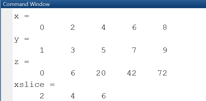
Im folgenden Beispiel werden drei anonyme Funktionen definiert.
- Zeile 1-3: Definiere die Funktion f(x) = sin(2πx) als anonyme Funktion und berechne die Funktionswerte in den Punkten x = 1 und x = 2.
- Zeile 4-8: Definiere das Polynom p(x) = 1 + 2x + x2 und berechne die Funktionswerte in den äquidistanten Punkten x = [0, 0.5, 1.0, 1.5, 2.0]. Da bei der Definition der Polynomfunktion der Punkt-Operator verwendet wird, darf ein Vektor als Argument der Funktion verwendet werden.
- Zeile 8-11: Definiere die dreidimensionale Funktion u(x,y) = 25xy, wobei x und y Vektoren derselben Länge sein müssen. Erzeuge dann zwei Vektoren x und y mit Hilfe der Funktion linspace und berechne die Funktionswerte z = u(x, y) mit Hilfe der anonymen Funktion.
% Beispiel 1: Sinus-Funktionf = @(x) sin(2*pi*x);y1 = f(1); y2 = f(2);% Beispiel 2: Polynomp = @(x) (1 + 2.*x + x.^2);x = 0:0.5:2; % x = [0, 0.5, 1.0, 1.5, 2.0]y = p(x);% Beispiel 3: Funktion mit zwei Variablenu = @(x,y)(25.*x.*y);x = linspace(0,1,10); y = linspace(0,2,10);z = u(x, y);
9 Plotting in MATLAB
Bei der numerischen Lösung eines mathematischen Problems wie z.B. einer partiellen Differentialgleichung ist es wichtig, Lösungen und Zwischenergebnisse einfach visualisieren zu können, da dies das intuitive Verständnis des zugrundeliegenden physikalischen Problems erleichtert. MATLAB verfügt über eine Reihe von Funktionen, die die Erstellung von zwei- und dreidimensionalen Grafiken unterstützen. Die wichtigsten Funktionen sind plot, surf, mesh, contour, quiver, diese sehen wir uns im Folgenden genauer an.
MATLAB-Grafiken sind in eigene Fenster eingebettet, die mit Hilfe des figure-Befehls erstellt werden. Ein Grafikfenster wird stets defaultmäßig erstellt, auch wenn der figure-Befehl nicht explizit angegeben wird. Der explizite figure-Befehl ermöglicht es, Optionen für die Erstellung des Grafikfensters anzugeben, z.B. Position und Titel.
9-1 2D-Plots mit plot
Die einfachste Grafik ist ein 2D-Linienplot, also eine zweidimensionale Liniengrafik einer Funktion y = f(x), wobei die Funktion plot() eingesetzt wird. Die plot-Funktion hat die allgemeine Syntax plot(X,Y), und erzeugt einen 2D-Linienplot der Daten in Y versus der entsprechenden Koordinaten in X. X und Y müssen Vektoren oder Matrizen derselben Größe sein. Um z.B. einen 2D-Plot der Funktion y = f(x) = x^2 für die Vektoren X = [1,2,3,4,5] und Y = [1,4,9,16,25] zu erstellen, schreibt man
plot([1,2,3,4,5], [1,4,9,16,25])
oder auch einfach
plot([1,4,9,16,25])
Fortgeschrittene Verwendung der plot()-Funktion ermöglicht die Angabe weiterer Eingabeparameter oder auch die Festlegung von Formatierungs-Optionen für die Grafik, die als Schlüssel-Wert-Paare angegeben werden.
Beispiel: 2D-Line-Plot
In diesem Beispiel untersuchen wir einige Optionen der Funktion plot und stellen die Sinus- und Kosinus-Funktion auf demselben Koordinatensystem dar.
- Zeile 2: Erstelle eine Diskretisierung x des Intervalls [-2*pi, 2*pi] mittels eines äquidistanten Vektors mit 51 Datenpunkten.
- Zeile 3 und 4: Berechne die y-Koordinaten für die zu zeichnenden Funktionen.
- Zeile 5: Erstelle eine neue Figur mit Breite 700 und Höhe 500 an der Position(50, 50).
- Zeile 6: Zeichne die sin-Funktion, die durch die Koordinaten x und y1 beschrieben wird.
- Zeile 7: Der Befehl hold on hält Grafiken im aktuellen Achsensystem fest, so dass neue Grafiken hinzugefügt werden können.
- Zeile 8: Zeichne die cos-Funktion, die durch die Koordinaten x1 und y2 beschrieben wird.
- Zeile 9-11: Gebe Titel, Legende und Achsenbeschriftungen an.
| Skript | Ausgabe |
|---|---|
|

|
In MATLAB können mit Hilfe der subplot-Funktion mehrere Grafiken in demselben Figurenfenster, jedoch auf unterschiedlichen Achsensysteme gezeichnet werden. Der Befehl subplot(m, n, p) teilt die aktuelle Figur in ein mxn Gitter aus Teilgrafiken, wobei der nächste plot an die Stelle p gesetzt wird.
Beispiel: 2D-Plot mit figure und subplot
Es sollen die Funktionen y1(x) = sin(x)*exp(x) and y2(x) = x*cos(x) auf derselben Funktion dargestellt werden, so dass die zweite Grafik unterhalb der ersten angeordnet ist. Um dies zu erreichen, wird mit dem Befehl subplot(2,1,p) ein Gitter mit zwei Zeilen und einer Spalte erstellt sowie ein Achsensystem an der Position p = 1,2, wie hier im Beispiel.
- Zeile 5: Erstelle subplot für die obere Grafik an Position p = 1
- Zeile 6-9: Erstelle Grafik mit plot die an der Stelle subplot p = 1 eingefügt wird. Linienstärke, Farbe und Marker werden als Schlüssel-Wert-Paare angegeben. Codezeile 6 wird mit Hilfe von Auslassungszeichen (...) geteilt.
- Zeile 10: Erstelle subplot für die untere Grafik an der Position p = 2
- Zeile 11-14: Erstelle Grafik mit plot die an der Stelle subplot p = 2 eingefügt wird.
| Skript | Ausgabe |
|---|---|
|

|
9-2 3D-Plots mit surf
Für die Erstellung dreidimensionaler Grafiken einer Funktion z = u(x,y) verwendet man in MATLAB die Funktion surf(). Die surf-Funktion hat die allgemeine Syntax surf(X, Y, Z), und erstellt ein Oberflächendiagramm der Daten in Z versus der Koordinaten in X und Y. Die Parameter X, Y und Z müssen Matrizen mit passenden Dimensionen sein. Die Matrizen X and Y werden aus den Koordinaten-Vektoren x and y mit Hilfe der Funktion meshgrid erzeugt. Falls x eine Vektor mit m Elementen und n ein Vektor mit n Elementen ist, erzeugt meshgrid(x, y) zwei Matrizen X and Y mit jeweils n Zeilen und m Spalten. X repliziert den Vektor x als Zeilenvektor n mal, und Y repliziert y als Spaltenvektor m mal.
Die folgenden Beispiele zeigen die Erstellung der Matrizen X, Y und Z, die als Parameter der Funktion surf benötigt werden, und allgemeiner die Verwendung der Funktionen meshgrid und surf.
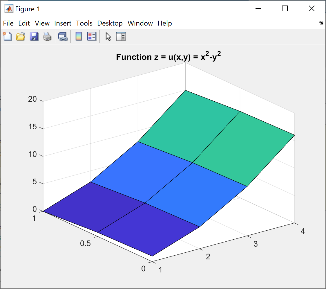
Beispiel: 3D-Plot mit surf
In diesem Beispiel erstellen wir ein Oberflächendiagramm der Funktion z = u(x, y) = x^2 - y^2 für gegebene x- und y-Koordinatenvektoren.
- Zeile 1-2: Erstelle Koordinatenvektoren x and y.
- Zeile 1-2: Die Koordinatenvektoren x and y werden als Eingabeparameter der Funktion meshgrid() verwendet um die Matrizen X und Y zu erzeugen.
- Zeile 4: Berechne die 3x4 Matrix Z, die die Funktionswerte enthält.
- Zeile 5: Erstelle Oberflächendiagramm mittels surf.
| Skript | Ausgabe |
|---|---|
Die Ausgabe im Kommandofenster ist wie abgebildet:
Output X, Y from meshgrid:
X =
     1     2     3     4
     1     2     3     4
     1     2     3     4
Y =
         0         0         0         0
    0.5000    0.5000    0.5000    0.5000
    1.0000    1.0000    1.0000    1.0000
Function values Z:
Z =
    1.0000    4.0000    9.0000   16.0000
    0.7500    3.7500    8.7500   15.7500
         0    3.0000    8.0000   15.0000
|
|
Beispiel 2: Gradientenfeld und Kontur-Plot visualisieren
Wir plotten die Funktion u(x,y) = x^2-y^2 über einen rechteckigen Wertebereich [a, b] x [c, d] und ergänzen die Grafik um Titel und Achsenbeschriftungen. Weiterhin zeigen wir die Konturlinien und das durch den Gradienten definierte Vektorfeld mit Hilfe der MATLAB-Funktionen contour and quiver.
- Zeile 1: Definiere u als anonyme Funktion.
- Zeile 2-3: Definiere das Rechteck [a, b] x [c, d] und die Anzahl nx = 10 and ny = 20 der Datenpunkte, die für die Diskretisierung verwendet werden sollen.
- Zeile 4: Erzeuge zwei Vektoren x und y mit äquidistanten Datenpunkten.
- Zeile 5: Erzeuge die Matrizen X, Y aus den äquidistanten x- und y-Koordinaten.
- Zeile 6: Berechne die Matrix Z, die die Funktionswerte enthält.
- Zeile 7: Berechne den Gradienten [px, py] der Funktion u.
- Zeile 9-13: Erstelle das Oberflächendiagramm der Funktion u.
- Zeile 14-20: Erzeuge 2D-plot der Funktion mit Konturlinien und Vektorfeld.
| Skript | Ausgabe |
|---|---|
|

|
10 Symbolische Berechnungen
Die Symbolic Math Toolbox dient der analytischen Analyse und Lösung mathematischer Probleme, beispielsweise zur Berechnung von Ableitungen, partiellen Ableitungen und Integralen von Funktionsausdrücken, zur Lösung von Gleichungen oder zur Darstellung von Funktionen. Der symbolische Modus wird durch die Eingabe des Schlüsselworts syms gefolgt vom Namen der symbolischen Variablen gestartet, zum Beispiel:
syms x
syms x y
syms x y z
Symbolische Berechnungen können interaktiv im Befehlsfenster oder in einem Skript durchgeführt werden. Die Ableitung einer Funktion wird mittels der Funktion diff, berechnet, das Integral mit der Funktion int und der Gradient mit Hilfe der Funktion grad. Für symbolische Plots gibt es eine Reihe von Funktionen wie fplot, fsurf und fcontour, deren Name mit "f" beginnt und die alle mit symbolischen Funktionsausdrücken arbeiten.
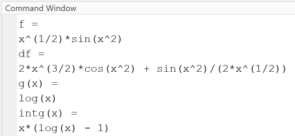
Das folgende Beispiel zeigt, wie man Funktionen einer Variablen deklariert und die Ableitung mit diff und das Integral mit int berechnet. Beachten Sie, dass der symbolische Modus in Zeile 1 mit dem Schlüsselwort syms und dem Namen der Variablen x und dann in Zeile 7 mit dem Schlüsselwort syms und dem Namen der Funktion g(x) gestartet wird.
| Skript | Ausgabe |
|---|---|
|
|
Autoren, Tools & Quellen
Autor:
Prof. Dr. Eva Maria Kiss
elab2go-Links:
- [1] MATLAB Live Scripts erstellen und verwenden: elab2go.de/demo-mat1/matlabLiveScripts.php
- [2] Demo-MAT3: Clusteranalyse "Automotive in 3D": elab2go.de/demo-mat3
- [3] Demo-MAT4: Predictive Maintenance mit MATLAB: elab2go.de/demo-mat4
Quellen:
- [1] MATLAB Hilfe: de.mathworks.com/help/matlab/
- [2] MATLAB Syntax Grundlagen: de.mathworks.com/help/matlab/language-fundamentals.html
- [3] Octave Software:www.gnu.org/software/octave/
- [4] Octave Manual:octave.org/doc/v6.1.0/